Compound Poisson-Normal Regression

Laszlo Pecze

2025-06-27

Introduction

In many applied settings—including insurance claims, biological systems, and environmental monitoring—the observed data arise from a random number of additive events, where each event contributes a continuous value. A natural model for such data is the Compound Poisson-Normal (CPN) distribution.

The CPN model assumes that the number of events follows a Poisson distribution, and that each event contributes an independent and identically distributed (i.i.d.) normally distributed amount.

Formally, let:

• $N \sim \text{Poisson}(\lambda)$ denote the number of events,
• $X_1, X_2, \ldots, X_N \overset{\text{i.i.d.}}{\sim} \mathcal{N}(\mu, \sigma^2)$, independent of $N$,

Then the total observed outcome is modeled as a compound sum:

$$Y = \sum_{i=1}^{N} X_i$$

The resulting distribution of $Y$ is known as the Compound Poisson-Normal distribution.

The first two moments of the CPN distribution are:

$$\mathbb{E}[Y] = \lambda \mu,\quad \text{Var}(Y) = \lambda (\mu^2 + \sigma^2)$$

These follow from the properties of the compound distribution, combining Poisson and Gaussian contributions. The (approximate) probability density function (pdf) of $Y$ is:

$$f_Y(y; \lambda, \mu, \sigma) = \begin{cases} e^{-\lambda}, & \text{if } y = 0 \\\\ \sum_{k=1}^{K_{\text{max}}} \frac{e^{-\lambda} \lambda^k}{k!} \cdot \frac{1}{\sqrt{2\pi k \sigma^2}} \exp\left( -\frac{(y - k\mu)^2}{2k\sigma^2} \right), & \text{if } y \neq 0 \end{cases}$$

Where:

• $y$: the observed total from the compound process
  
• $\lambda$: expected number of Poisson events
  
• $\mu$: mean of each normal component
  
• $\sigma$: standard deviation of each normal component
  
• $k$: number of events (from 1 to $K_{\text{max}}$)
  
• $K_{\text{max}}$: maximum number of events used in the approximation

When $k = 0$, the sum is defined as a point mass at zero, and its probability is:

$$P(Y = 0) = P(N = 0) = e^{-\lambda}$$

In theory, the compound distribution sums over an infinite range of possible Poisson event counts. In practice, this sum must be truncated at a finite maximum value $K_{\max}$, chosen so that the remaining tail probability is negligible.

Getting Started

To use the function, load the package:

library(CPN)

Simulating Data

We’ll simulate a dataset that mimics typical CPN behavior. This includes both categorical and continuous predictors, and outcomes generated via a Poisson count of normally distributed values.

set.seed(123)
data <- simulate_cpn_data()
head(data)
#            y x1          x2
# 1 -0.5703738  A  0.25331851
# 2  0.0000000  A -0.02854676
# 3  0.9613621  A -0.04287046
# 4  5.3350483  B  1.36860228
# 5  3.1328607  A -0.22577099
# 6 -2.6186645  B  1.51647060

Plot the simulated data

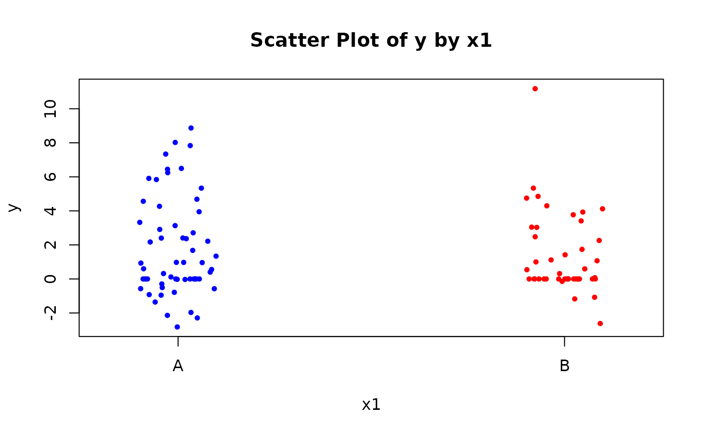
Visualize the response y against predictor x2, colored by group x1.

# Scatter plot of y vs x1
stripchart(
  y ~ x1, data = data,
  vertical = TRUE, method = "jitter",
  pch = 19, cex = 0.6,
  col = c("blue",  "red"),
  xlab = "x1", ylab = "y",
  main = "Scatter Plot of y by x1"
)

Fit the CPN Model

Fit a Compound Poisson-Normal regression model to the data using a standard formula interface. The response variable y is modeled as a function of predictors x1 (categorical) and x2 (continuous).

fit <- cpn(y ~ x1 + x2, data = data)

Summary of Results

Get a summary of the fitted model, including coefficient estimates, standard errors, z-values, and p-values. The summary also includes estimates of the mu and sigma parameters (mean and SD of the normal component) and model fit statistics like AIC.

summary(fit)
# Call:
# cpn(formula = y ~ x1 + x2, data = data)
# 
# Deviance Residuals:
#    Min     1Q Median     3Q    Max 
# -2.871 -2.059 -1.269  2.181  3.745 
# 
# Coefficients:
#             Estimate Std.Error z.value      Pr.z    
# (Intercept)  0.63754   0.15190  4.1969 2.705e-05 ***
# x1B         -0.60713   0.22934 -2.6473  0.008114 ** 
# x2           0.53609   0.10791  4.9679 6.767e-07 ***
# ---
# Signif. codes:  0 '***' 0.001 '**' 0.01 '*' 0.05 '.' 0.1 ' ' 1
# 
# Estimated mu parameter: 0.9600
# Estimated sigma parameter: 1.7062
# 
# Null deviance: 478.20 on 99 degrees of freedom
# Residual deviance: 449.74 on 95 degrees of freedom
# AIC: 459.74

Extracting Model Components

You can directly access key components of the fitted model object:

fit$coefficients
# (Intercept)         x1B          x2 
#   0.6375359  -0.6071284   0.5360923
fit$mu
#        mu 
# 0.9599623
fit$sigma
#    sigma 
# 1.706243
fit$fitted_values[1:10]  # preview only
#  [1] 2.0802264 1.7884887 1.7748077 2.0611074 1.6090445 2.2311441 0.4313962
#  [8] 1.3538511 1.9407450 2.0389587

Coefficients and Interpretation

Use coef() to extract model coefficients. Setting full = FALSE shows only the linear predictor coefficients (excluding auxiliary parameters like mu and sigma).

coef(fit)
# (Intercept)         x1B          x2          mu       sigma 
#   0.6375359  -0.6071284   0.5360923   0.9599623   1.7062428
coef(fit, full = FALSE)  # Includes only linear predictors
# (Intercept)         x1B          x2 
#   0.6375359  -0.6071284   0.5360923

Diagnostics and Residuals

Basic diagnostic plots and residuals help check model fit and detect issues like non-linearity or outliers.

plot(fit)

residuals(fit)[1:10]
#  [1] -2.215482 -1.930328 -1.997946  2.411580  2.145066 -2.766042  2.737024
#  [8]  2.297386 -2.398468 -2.008626

Likelihood and Information Criteria

These metrics are useful for comparing model fit. logLik() gives the log-likelihood, AIC() the Akaike Information Criterion (lower is better), and vcov() returns the variance-covariance matrix of the parameters.

logLik(fit)
# 'log Lik.' -224.8705 (df=5)
AIC(fit)
# [1] 459.741
vcov(fit)
#              (Intercept)          x1B           x2           mu        sigma
# (Intercept)  0.023075014 -0.018395473 -0.002512385 -0.010214396 -0.007321724
# x1B         -0.018395473  0.052596614  0.000287386  0.002777711 -0.001478573
# x2          -0.002512385  0.000287386  0.011644724 -0.002747529 -0.001565976
# mu          -0.010214396  0.002777711 -0.002747529  0.027438819  0.008114203
# sigma       -0.007321724 -0.001478573 -0.001565976  0.008114203  0.033661888

Type I Analysis of Deviance

The function anova(fit) provides a sequential (Type I) analysis of deviance.
This examines the incremental contribution of each predictor to the model’s fit, based on the order in which they appear in the formula.

anova(fit)
#       Term     Df Deviance Resid. Df Resid. Dev   Pr(>Chi) Signif
#  Residuals                        97      478.2                  
#         x1      1   6.7993        96      471.4  0.0091193     **
#         x2      1   21.657        95     449.74 3.2607e-06    ***
# ---
# Signif. codes:  0 '***' 0.001 '**' 0.01 '*' 0.05 '.' 0.1 ' ' 1

Model Update and Comparison

You can update a model (e.g., remove predictors) and compare nested models using the likelihood ratio test:

fit2 <- update(fit, . ~ . - x2)

anova(fit, fit2)  # Likelihood ratio test
#    Model Resid. Df Resid. Dev     Df Deviance   Pr(>Chi) Signif
#  Model 1        95     449.74                                  
#  Model 2        96      471.4      1   21.657 3.2607e-06    ***
# ---
# Signif. codes:  0 '***' 0.001 '**' 0.01 '*' 0.05 '.' 0.1 ' ' 1

Prediction

Once you have fitted a Compound Poisson-Normal (CPN) regression model using the cpn() function, you can generate predictions on both the original data and new observations using the predict() method for cpn objects.

This method supports three prediction types:

• “link”: Returns the linear predictor $\eta = X\beta$.
• “rate”: Returns the rate component $\exp(\eta)$, representing the expected number of latent events.
• “response”: Returns the expected response $\mathbb{E}[Y] = \mu \cdot \exp(\eta)$, combining the frequency and magnitude components of the compound distribution.

Additionally, confidence intervals can be requested using the interval = "confidence" argument, which computes approximate normal-theory confidence intervals using the delta method.

Predicting on the Original Data

By default, predict() uses the original dataset used for model fitting. You can obtain point estimates or confidence intervals for the fitted values.

# Point predictions on the response scale
predict(fit, type = "response")[1:5]
# [1] 2.080226 1.788489 1.774808 2.061107 1.609045

# Confidence intervals for response predictions
predict(fit, type = "response", interval = "confidence")[1:5, ]
#        fit       lwr      upr
# 1 2.080226 1.1475902 3.012863
# 2 1.788489 0.9814659 2.595511
# 3 1.774808 0.9733248 2.576291
# 4 2.061107 0.8876666 3.234548
# 5 1.609045 0.8722838 2.345805

Predicting on New Data

To make predictions on new data, provide a data.frame to the newdata argument. The function will internally align factor levels and construct the appropriate model matrix.

# Define new observations
new_df <- data.frame(
  x1 = c("A", "A", "B", "B"),
  x2 = c(-0.5, -0.2, -0.3, -0.3)
)

# Predictions on the link scale (linear predictor η)
predict(fit, newdata = new_df, type = "link", interval = "confidence")
#          fit         lwr       upr
# 1  0.3694897  0.03861794 0.7003615
# 2  0.5303174  0.22324817 0.8373866
# 3 -0.1304202 -0.52855693 0.2677165
# 4 -0.1304202 -0.52855693 0.2677165

# Predictions on the rate scale (exp(η))
predict(fit, newdata = new_df, type = "rate", interval = "confidence")
#         fit      lwr      upr
# 1 1.4469960 1.039373 2.014481
# 2 1.6994716 1.250131 2.310321
# 3 0.8777265 0.589455 1.306976
# 4 0.8777265 0.589455 1.306976

# Predictions on the response scale (μ × exp(η))
predict(fit, newdata = new_df, type = "response", interval = "confidence")
#         fit       lwr      upr
# 1 1.3890617 0.7318477 2.046276
# 2 1.6314287 0.8861812 2.376676
# 3 0.8425844 0.4024248 1.282744
# 4 0.8425844 0.4024248 1.282744

Confidence Intervals

When interval = "confidence" is used:

• On the link and rate scales, confidence intervals are based solely on the uncertainty in the regression coefficients ($\beta$).
• On the response scale, the intervals additionally incorporate uncertainty in the mean magnitude parameter ($\mu$) using the delta method:

$$\text{SE}[\mu \cdot \exp(\eta)] \approx \sqrt{(\mu \cdot \exp(\eta))^2 \cdot \text{Var}[\eta] + (\exp(\eta))^2 \cdot \text{Var}[\mu]}$$

This provides a more accurate reflection of total uncertainty when predicting expected values of the compound outcome.

```

Conclusion

The CPN package enables effective modeling of semicontinuous data using the Compound Poisson-Normal model. It supports flexible model specification, S3 methods for diagnostics and inference, and prediction on new data. For more advanced use, refer to the function documentation or the package reference manual.

References

D. C. Nascimento, Abraão, Leandro C. Rêgo, and Raphaela L. B. A. Nascimento. 2019. “Compound Truncated Poisson Normal Distribution: Mathematical Properties and Moment Estimation.” Inverse Problems &Amp; Imaging 13 (4): 787–803. https://doi.org/10.3934/ipi.2019036.

Hu, Haoran, Xinjun Wang, Site Feng, Zhongli Xu, Jing Liu, Elisa Heidrich-O’Hare, Yanshuo Chen, et al. 2024. “A Unified Model-Based Framework for Doublet or Multiplet Detection in Single-Cell Multiomics Data.” Nature Communications 15 (1): 5562.

Raqab, Mohammad Z, Debasis Kundu, and Fahimah A Al-Awadhi. 2021. “Compound Zero-Truncated Poisson Normal Distribution and Its Applications.” Communications in Statistics-Theory and Methods 50 (13): 3030–50.